The GUI (graphical user interface) of the Eliko RTLS Manager can be used to configure basic RTLS settings and visualize the anchors and tags in real time.
Connecting to Eliko RTLS Manager
In case of a standalone RTLS Server machine, there are three options to access the Eliko RTLS Manager web interface.
Option 1: Wi-Fi connection
For connecting a Wi-Fi enabled laptop, which is located close enough to the RTLS Server machine, the easiest way is using the wireless network provided by the RTLS Server. The name of this network may be Eliko-RTLSS-BS-XXXX, KIORTLSS-BS-XXXX or KIORTLSS-AP- XXXX, where XXXX is a 4-digit number which is unique among all the RTLS Server machines. Just look this network up on your laptop and create a connection to it. This connection is protected by a password, which you can find as a sticker on the bottom of the RTLS Server machine. NB! Please note that on some operating systems, a laptop will assume it gets internet access through this Wi-Fi connection, which is not true. After clicking “connect” on the laptop, it may be shown for quite a long time that establishing the connection is still in progress, while the connection is actually created with a couple of seconds. This means it would be OK to verify the connection just a couple of seconds after clicking the “connect” button, without waiting for the progress indicator to finish.
When connected via Wi-Fi, you can access the Eliko RTLS Manager web interface by using your web browser to access the following URL: http://10.8.4.1 with the RTLS Web UI access credentials provided by Eliko.
Option 2: Cable-based Ethernet connection via Anchor Network port
For a cable-based Ethernet connection, the easier way is to connect the PC behind the Anchor Network and leave the Client Network unused. The PC should be configured to obtain an IP address from an external DHCP server (this configuration may already be the default one). If the RTLS anchors are connected via Wi-Fi, the Anchor Network port of the RTLS Server machine (“ETH_A”) is empty and a simple ethernet cable may be used to connect the PC. If the Anchor Network port is already occupied by a network switch, then the PC should be connected behind any switch residing in the Anchor Network. Please note that PoE functionality is not required for connecting a PC, so you can also use a non-PoE port for this connection.
As in case of Wi-Fi, you can just use your browser to access the following URL: http://10.8.4.1 with the RTLS Web UI access credentials provided by Eliko.
Option 3: Cable-based Ethernet connection via Client Network port
It is also possible to connect a PC directly to the Client Network port (“ETH_C”), but this may be more complicated to configure. The Client Network interface expects an external
DHCP server to lease an IP address to the RTLS Server. With the current case, the client’s PC should have a DHCP server running for this purpose. When connecting via the Client Network port, you can’t access the same URL as mentioned in two previous options. You need to use the admin panel of your DHCP server to find the IP address it has leased to the RTLS Server. You can then access the RTLS Manager web interface by using your web browser and this IP address as the URL.
If you connect the Eliko RTLS Server’s “Client Network” port to your company’s network router and your network has a DHCP server running, you can also access the RTLS Server from your PC connected to the company’s network without connecting it directly to the Client Network (“ETH_C”) port of the RTLS server machine. You need to access the admin UI of your network router in order to look up for the IP address leased by your network’s DHCP server to the RTLS Server. This IP address can then be used to access the Eliko RTLS Manager web interface from your PC connected to your network. As in case of two previous options, you need to use the RTLS Web UI access credentials provided by Eliko.
Web UI menu
When you access the RTLS Manager Web UI, the following sections of the menu should appear (more details are given in the next 4 subsections):
-
Map: start page by default. Here you can add and scale floorplan images, visualize anchors and tags.
-
Anchors: contains a list of anchors and their status. It is possible to configure the anchor’s coordinates, label (text alias) and add it to an area.
-
Tags: contains a list of tags, their status and battery level indication. It is possible to configure the tag’s positioning mode (2D or 3D), fixed height, alias name and reporting interval values.
-
RTLS Settings: currently this section only contains the System Accuracy Verification functionality
-
System: a large section containing settings for floorplan images, anchor groups and a separate admin tool for user and user group management.
Map view and layout plan
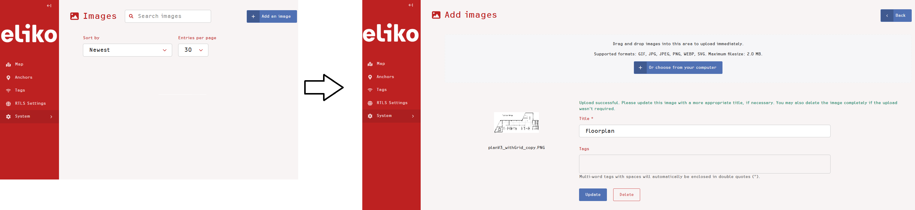
To upload floorplan images, choose the “System” section from the left menu and then choose “Images” → “Add an image” (Figure 5.1). Supported file formats are GIF, JPG, JPEG, PNG, WEBP and SVG; maximum file size is 2 MB.
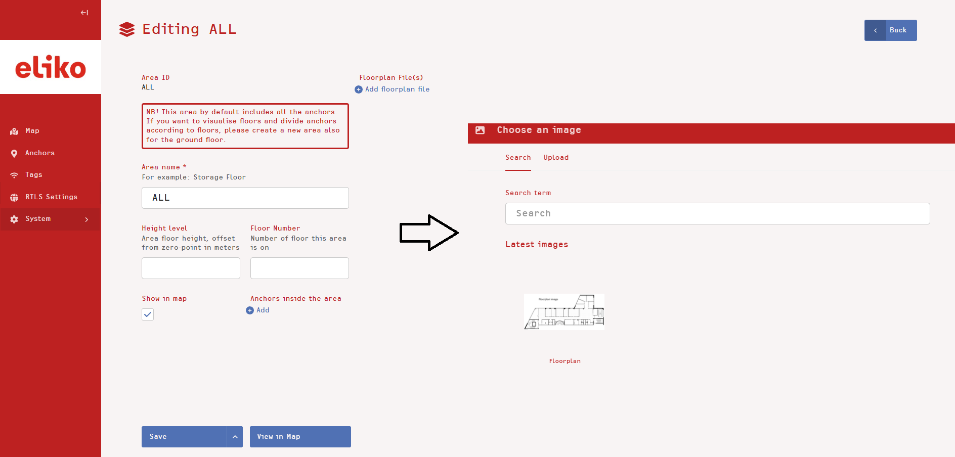
To make your floorplan visible in Map view, choose the “System” section from the left menu and then choose “Areas”. By default, you will see the “ALL” area in the list; you may later create your own areas and associate other floorplan images with them, which is useful in case of a multi-floor setup (for more information about areas please see the “Managing areas” subsection). To associate your floorplan with an area, press “Edit” next to your area, then press “Add floorplan file” and choose your recently updated floorplan from the menu (Figure 5.2). After applying your changes, you will see the uploaded floorplan in your map view.
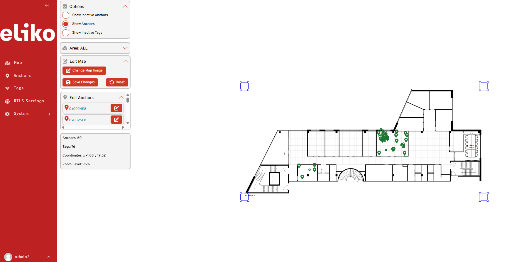
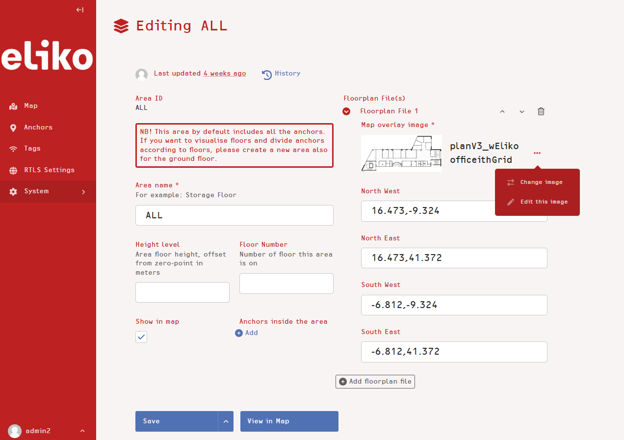
You can reposition and scale a floorplan image in the map view by pressing “Reposition and Scale Map” in the “Edit Map” section of the Map view menu (Figure 5.3). By moving the floorplan image you can adjust its position with regards to the coordinate zero point, while by dragging the blue squares in the edges of the image you can adjust the floorplan image scale. After you save your changes by clicking the “Save changes” button, you can check if the image is associated with its area and see the coordinates of your edge points that appear in the respective area window (see an example for “ALL” in Figure 5.4). Tip: you can write down these coordinates or save a screenshot of the UI view to be able to restore the configuration, should a file be lost or deleted by a mistake.
Anchors
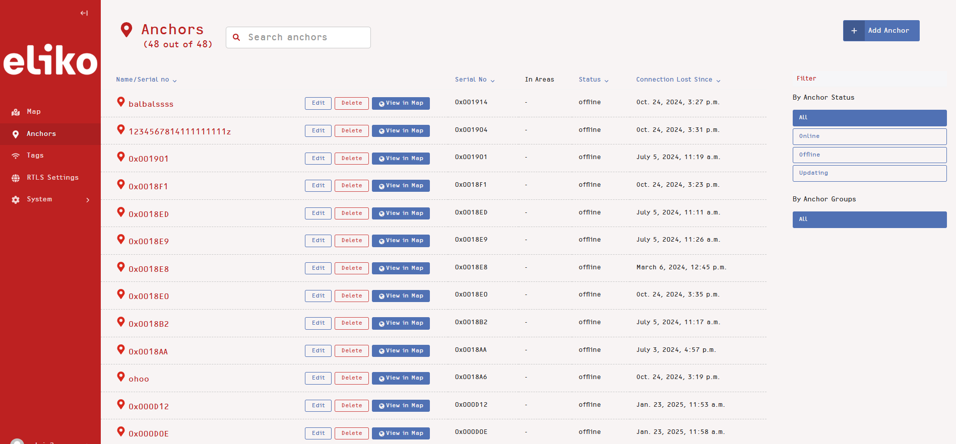
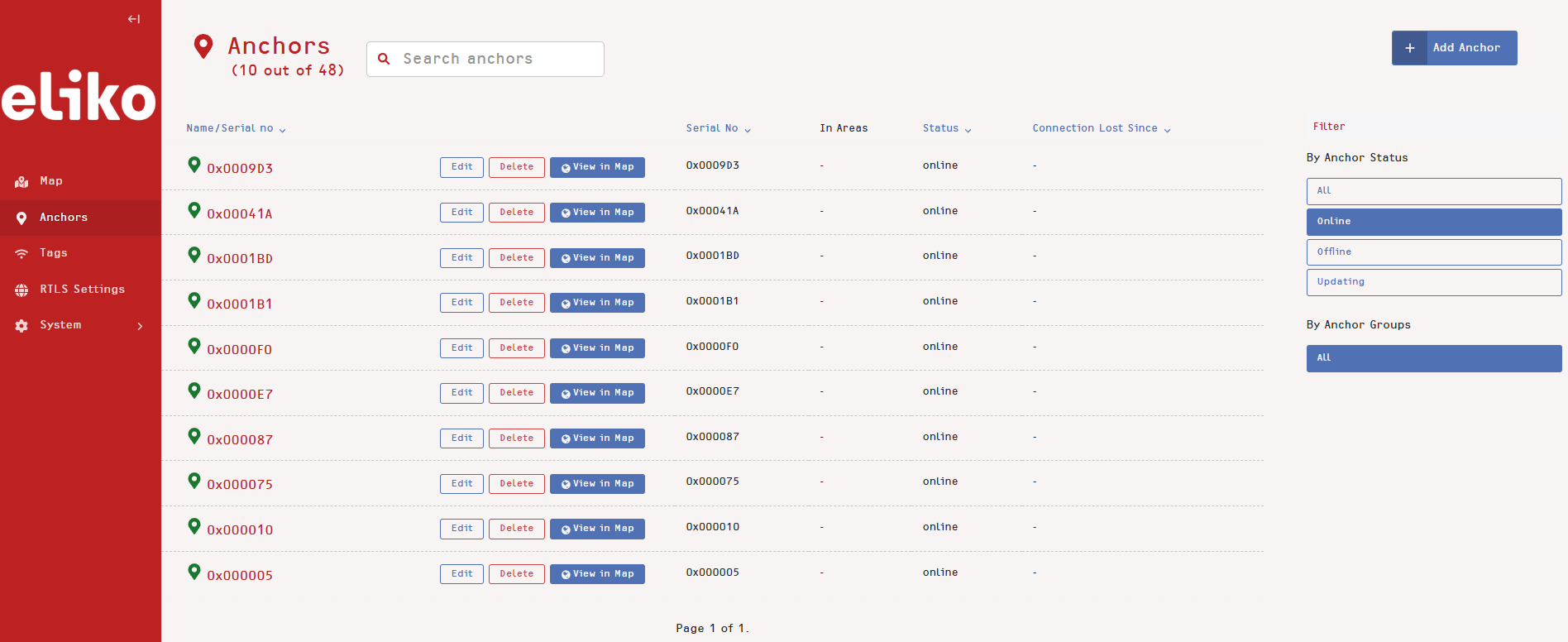
In the “Anchors” section of the UI menu you should see a list of all of the anchors with their serial numbers and/or labels (alias names) that are connected to the system. The green or red pinpoint in front of each anchor indicates if it is on- or offline. Status filters from the right side menu can be applied to the anchors' list (in Figure 5.5 all anchors are visualized by default, while Figure 5.6 shows only a list of active anchors). A search window in the upper part of the anchors' list can be used to find a particular anchor by its serial number or label.
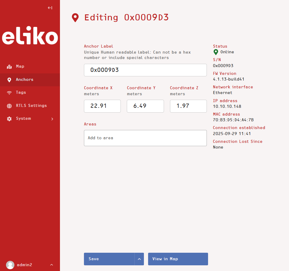
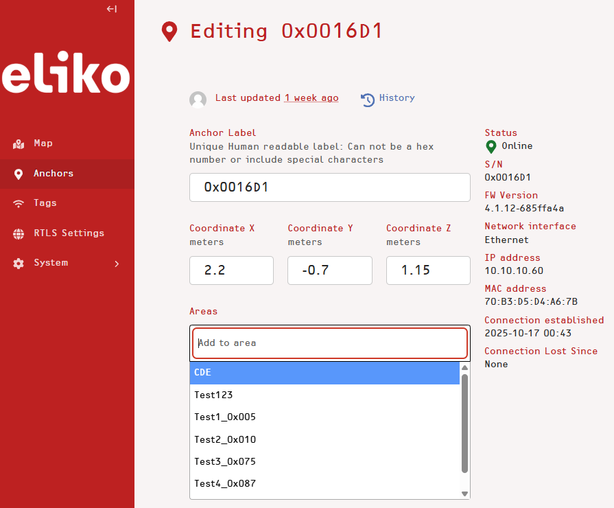
To adjust the anchor coordinates, click the “Edit” button of the desired anchor in the list and the “Editing anchor” page will appear (Figure 5.7). On this page you can insert the values of X, Y and Z coordinates in meters into the appropriate windows. You can also set up a label for each anchor in the same view. To save the settings, press the “Save” button.
To visualize the anchor’s position on the tracking area map, you can press the “View in Map” button of the desired anchor either in the anchors list or on the particular anchor’s page. You will get redirected to the map view centered according to the desired anchor’s coordinates.
To add anchor to an area (anchor group), select an area from the “Areas” dropdown menu. For more details about areas please refer to the “Managing areas” subsection.
Tags
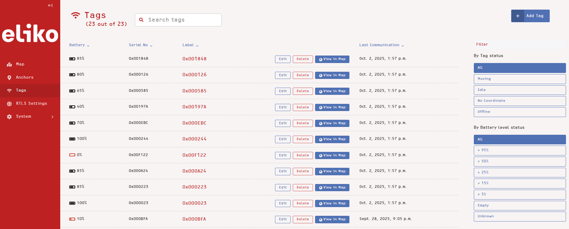
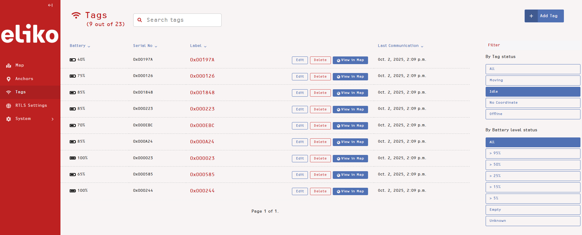
The tags section gives you an overview of all the tags that have been connected to the system. In this list you can see tag serial numbers, aliases, their battery levels and last communication time with the system (see Figure 5.8). Similar to anchors list, you can apply a filter from the menu on the right; tag status and battery level can be used for filtering (see idle tags example in Figure 5.9). Offline tags show the date and time of when the last coordinate was calculated.
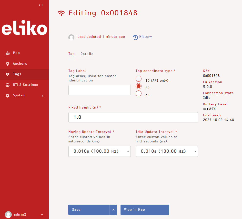
To adjust the tag settings, click the “Edit” button of the desired tag in the list and the “Editing tag” page will appear (Figure 5.10). You can configure the following settings:
-
Tag label: a human-readable text alias used in the system with the serial number. This parameter is optional.
-
Tag positioning mode (displayed as “Tag coordinate type”): currently, only 2D and 3D options are available
-
Tag fixed height: if positioning mode is set to 2D, a data field with the fixed tag height value appears on the page. For more accurate 2D positioning, it is recommended to set this value as close to the real height of the tag as possible. In case of 3D positioning this parameter becomes irrelevant.
-
Moving and idle update intervals: the location data is received with high update interval while the tag is moving, and when it stays stationary it will reduce the update rate to the level of low update interval. The interval values are set up in milliseconds and can be either entered manually or selected from the drop-down menu with pre-defined values. The minimum and maximum reporting interval values are 10 ms and 60000 ms, respectively. Please note that high (moving) update interval can only be smaller or equal to low (idle) update interval.
To save the tag settings, press the “Save” button.
To visualize the tag’s position on the tracking area map, you can press the “View in Map” button of the desired tag either in the tags list or on the particular tag’s page. You will get redirected to the map view centered according to the desired tag's coordinates. Please note that offline tags are not displayed in the map view by default, you should select the option “Show inactive tags” in the left side menu, which will visualize the tag’s last reported position before going offline.
RTLS Settings
Currently, the RTLS section of the UI menu contains the System Accuracy Verification feature. The same procedure can also be done via API, for more details please refer to the “System Accuracy Verification” section of the Eliko API manual.
Accuracy verification
Before you start the verification process, it is recommended to make the following preparations:
-
Select reference points in your tracking area and precisely measure their X, Y and Z coordinates by a laser tool. In these points the tag performing verification measurements should be visible to anchors. A good practice is to select items or surfaces above the floor level that are suitable to put a tag where it can be standstill during a test. Please note that you also need to define the order of the reference points from the first one to the last one: you will further need to make the measurements in the same order as you have defined.
-
Select a tag to be used for reference tests. Make sure it has a sufficient battery level and its reporting intervals are not too long (<1s).
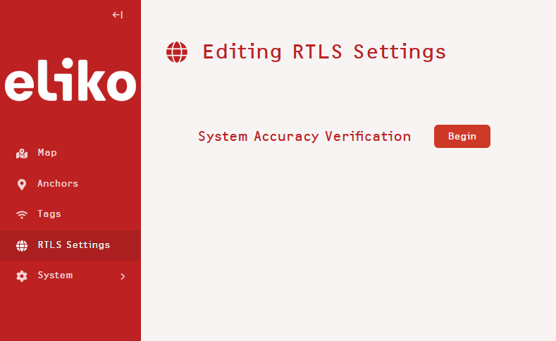
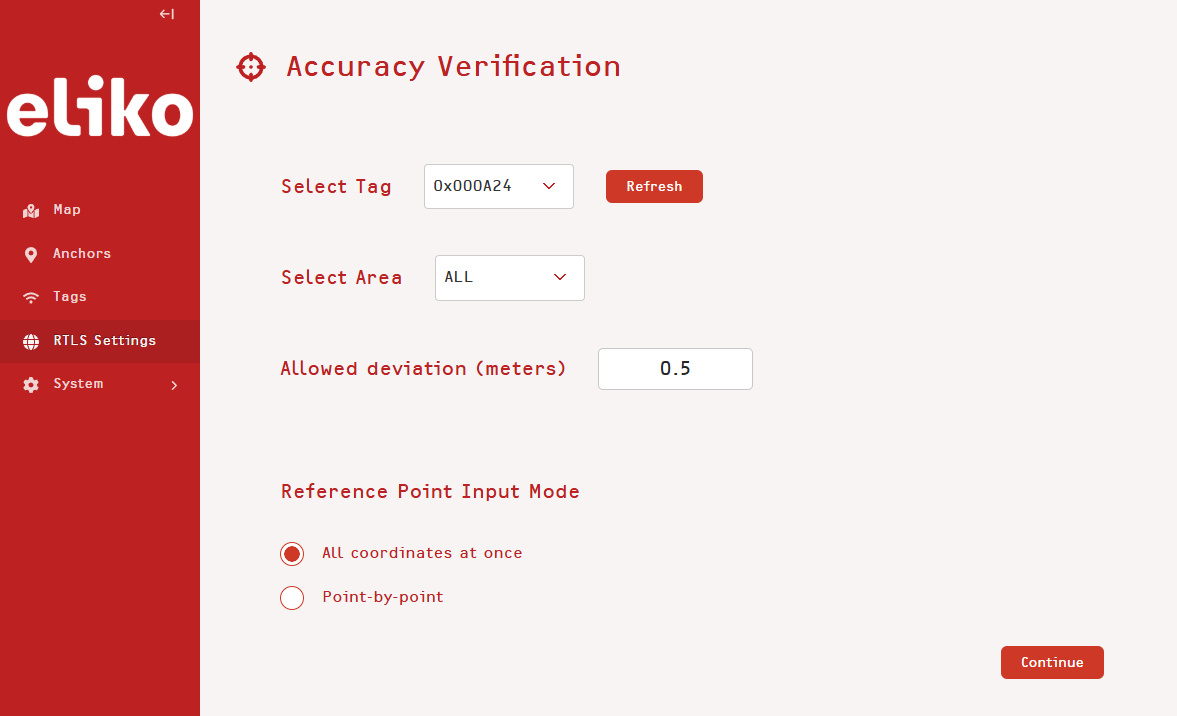
The process starts with selecting “System Accuracy Verification” from the “RTLS Settings” tab of the UI menu and pressing the “Begin” button (Figure 5.11). Next step is to select the serial number of your tag chosen for the tests and set up a value for allowed deviation (in meters), which will be the accuracy criteria. Then, you can choose between two reference point input modes: all coordinates at once or point-by-point and press “Continue” (Figure 5.12). This manual will guide you through both options.
All coordinates at once
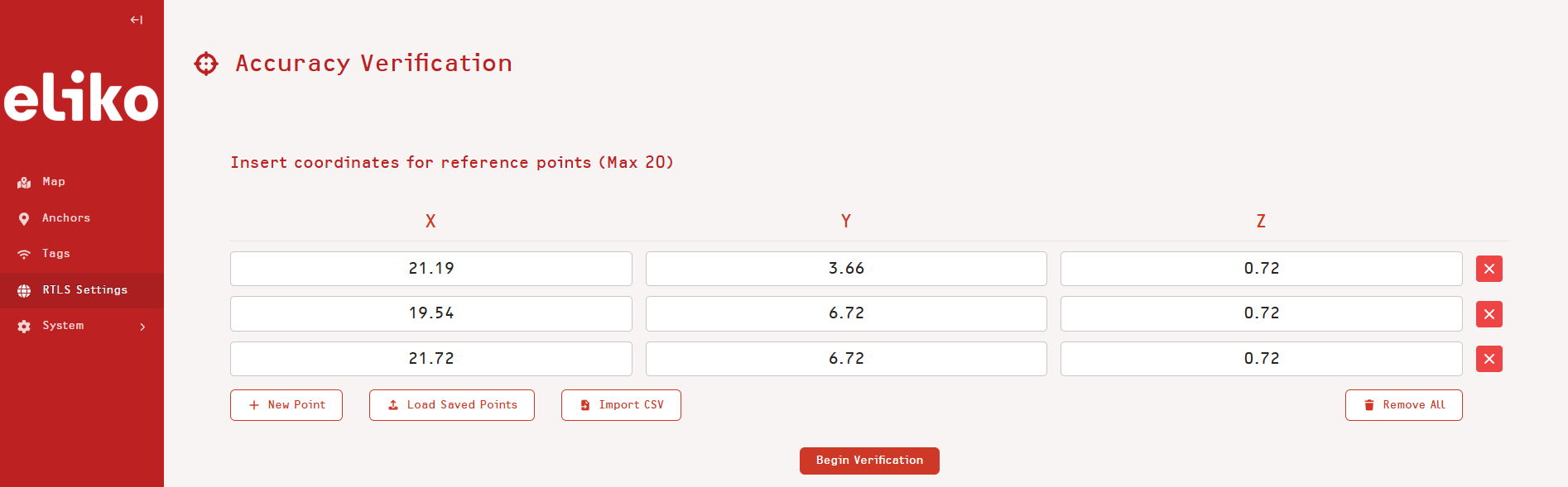
If you select “All coordinates at once”, you will have to enter or import the coordinates of all of your reference points (Figure 5.13). To enter the coordinates, fill the X, Y and Z coordinate fields of each point, from the first to the last, according to the order that you have defined. Another option is to import the coordinates in CSV format, where the file should only contain the values of X, Y and Z coordinates of each reference point given in the same order as you want to make the tests, i.e. from the first to the last. If you have saved a set of measurement points from the previous test, you can also use the option “Load Saved Points”.
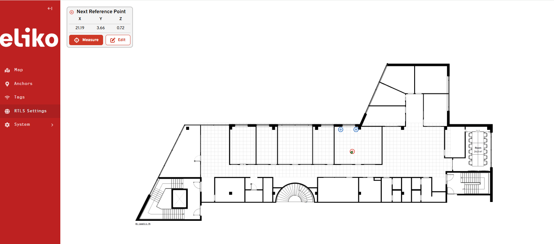
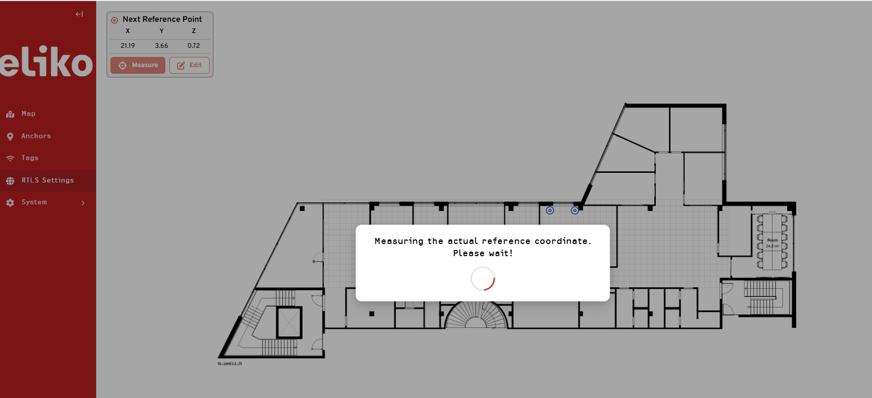
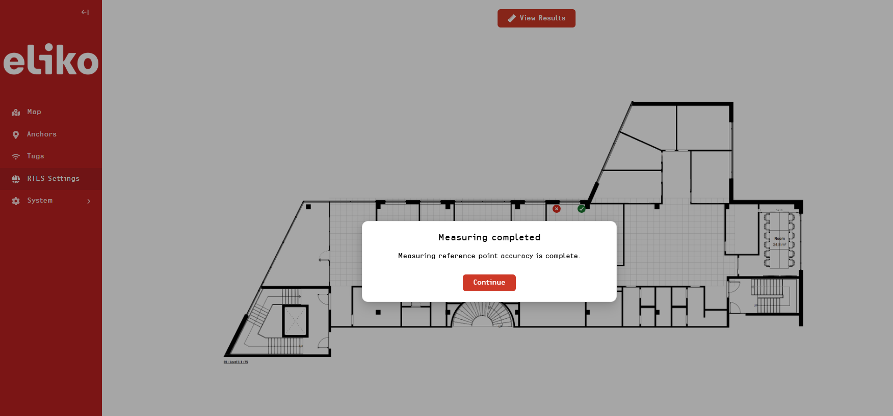
After all reference points are selected, press “Begin Verification” to proceed and you will see a map view with your imported reference points displayed as concentric circles (Figure 5.14). You will then need to start accuracy verification measurements by locating your selected tag in the first reference point. Make sure that your tag is displayed correctly in the UI map view with respect to its current reference point, as seen in Figure 5.14. When you are ready to start your measurements, press the “Measure” button in the reference point menu in the upper-left corner. You will then need to wait for some seconds (Figure 5.15; the longer the tag’s reporting interval, the longer the waiting time) until the next reference point measurement window will appear (Figure 5.16). Repeat the same procedure in each reference point.
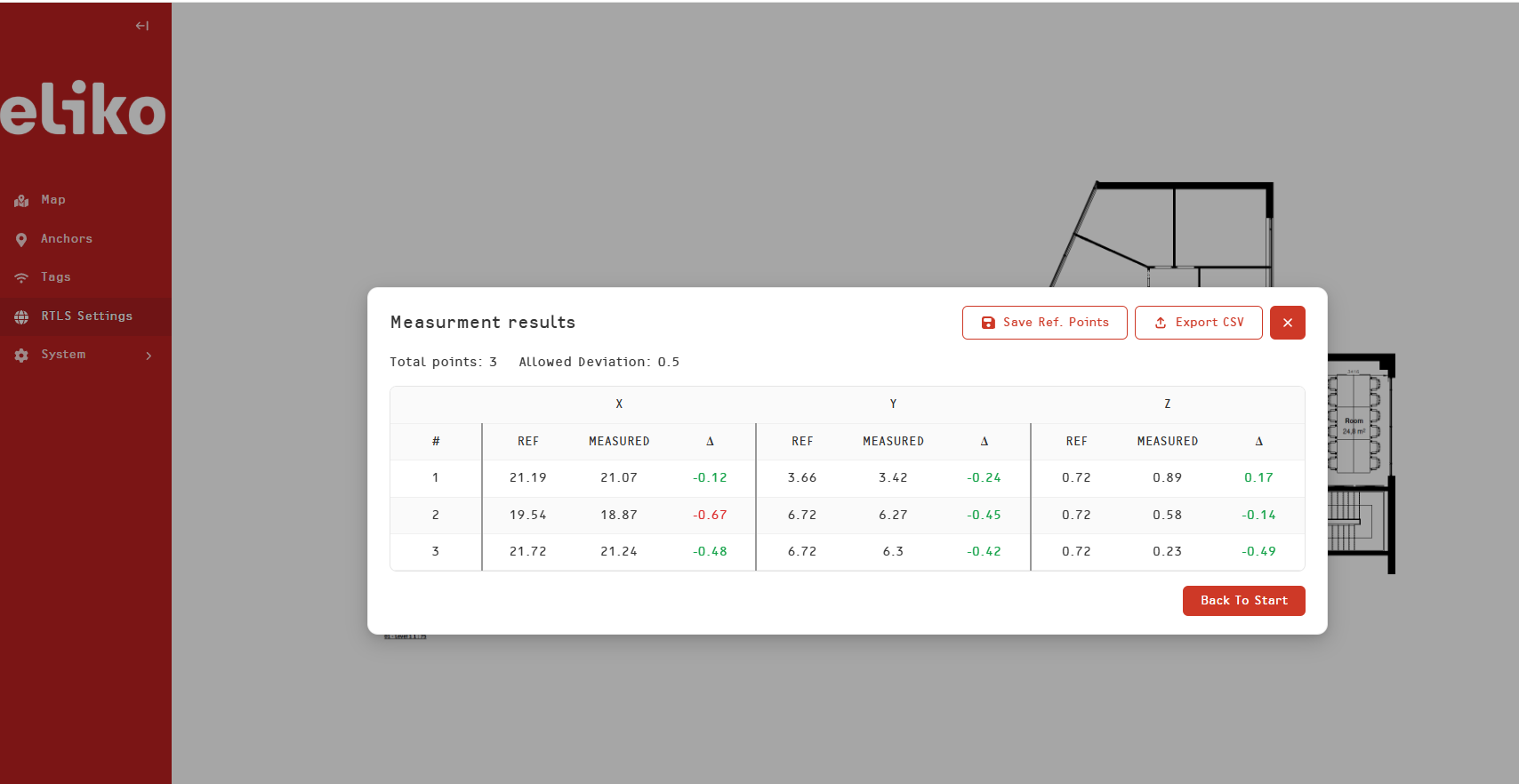
When the measurement in your last reference point is completed (Figure 5.17), an accuracy verification report is generated (Figure 5.18). For each reference point this report contains its known and measured X, Y and Z coordinates and their difference (delta). If the delta value is within the allowed deviation limits, it is displayed in green, otherwise it is displayed in red. From this view it is also possible to:
-
Save the reference points so that they can be used next time. Please note that if you choose and save a different set of reference points next time, your previous reference point set will be overwritten.
-
Export your report results into CSV
Point-by-point
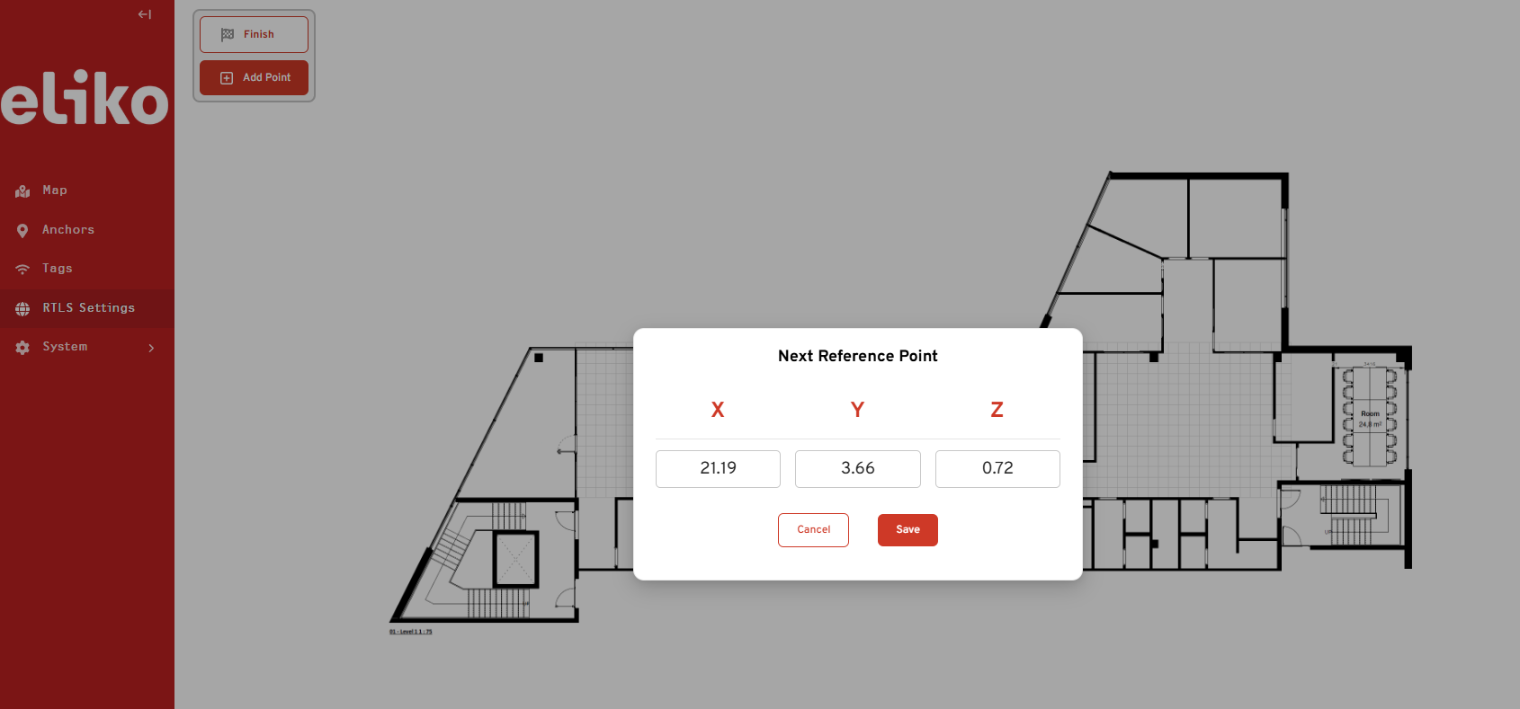
If you select the “Point-by-point” option, you will have to repeat the same procedure for each of your reference points:
-
Enter the X, Y and Z coordinates and press “Save” in a dialog box (Figure 5.19)
-
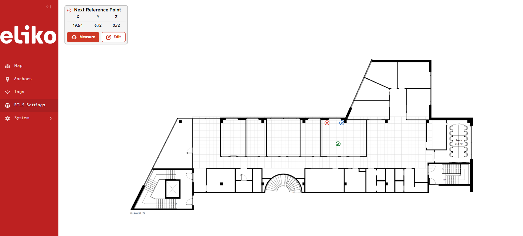
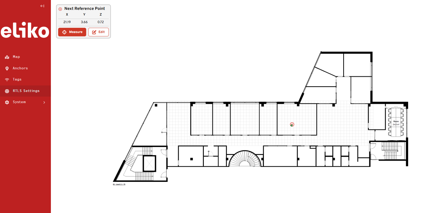
Press “Measure” in the upper left “Next Reference Point” menu tab that appears in the Map view (Figure 5.20)
-
Wait until the measurement is completed and a dialog box to insert the coordinates of your next reference point appears.
If you have finished your measurements, press “Cancel” in the next reference point’s dialog box and then press “Finish” in the upper left menu tab that appears in the Map view. Then, the system generates an accuracy report with the same data, structure, visualization and saving/exporting possibilities as in case of “All coordinates at once” option.
System
In the “System” section of the Web UI menu you can manage:
-
Floorplan images, as already described in the “Layout plan” section
-
Areas: this can be useful in case of a multi-floor setup, when you can define floorplan images for different floors. It is also possible to associate anchors with areas by means of anchor group feature.
Managing areas
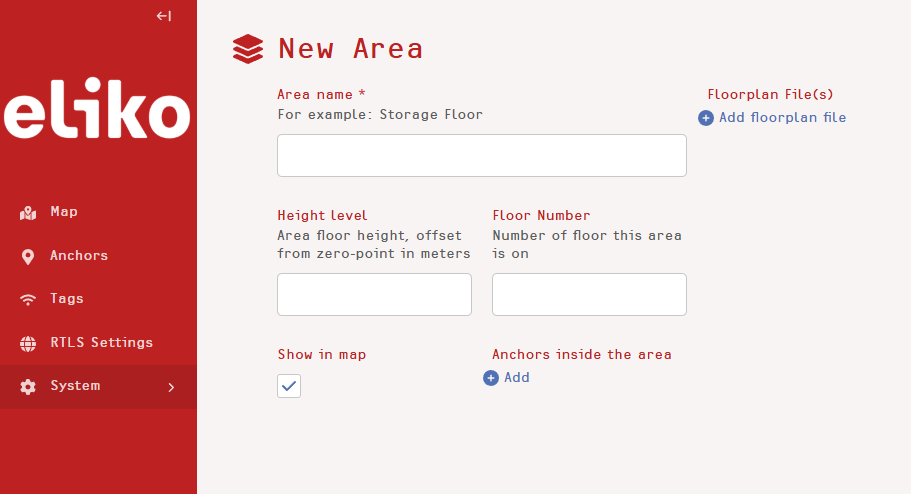
To visualize your areas, go to “Stsyem” → “Areas”, by default the area “ALL” must be present. To add an area, press “Add area” and then insert the following data (Figure 5.21):
-
Area name (mandatory)
-
Height level
-
Floor number
To add a floorplan image, press the “Add floorplan file” in the “New Area” view, select your image and save your settings, just as described in the “Map view and layout plan” section above. In a similar way as for the default area “ALL”, the new area floorplan image can be repositioned and rescaled.
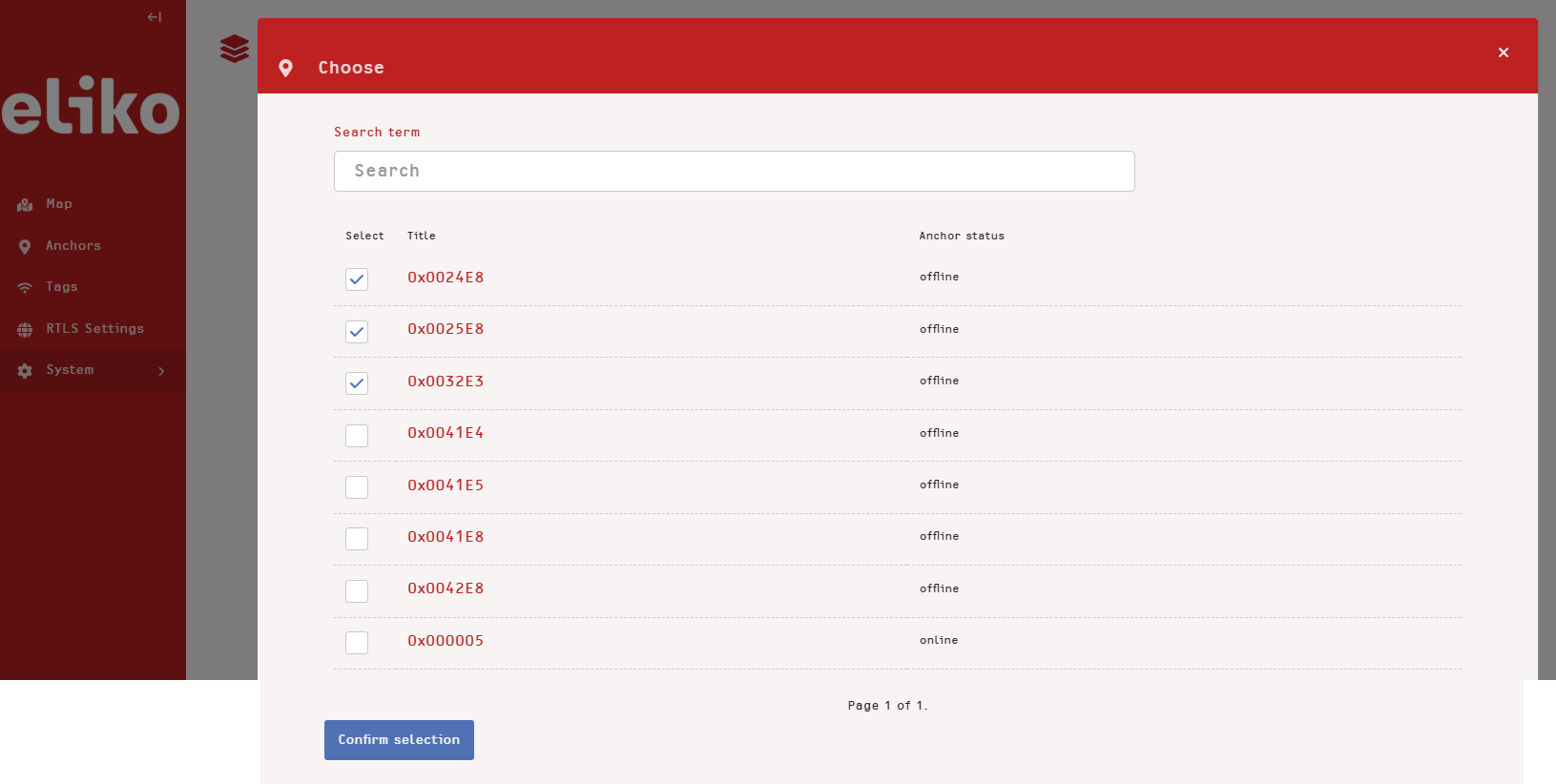
To add anchors to your area, press “Add” under the “Anchors inside the area”, select a list of anchors from the menu and press “Confirm selection” (Figure 5.22). Alternatively, you can assign anchors to an area when editing individual anchor’s data; in this case select an area from the “Areas” dropdown menu (Figure 5.23).
The floorplan, anchors and tags located in each area can be visualized in the Map view, just select your area instead of “ALL” from the area list in the left menu, as described in the “Map view and layout plan” section above.